Sunday, October 17, 2010

How To Make A Wrestling Kick Pads

Struccante Clinique Rinse-off Foaming Cleanser

  • Some time ago I managed to
  • obtain two samples of this cream blush in
  • of MUFE. I was curious to try it and I was strongly attracted by the wide range of colors (14).
  • HD Blush is a cream blush That naturally the highlights and sculpts cheeks for a healthy glow. Its mattifying and Reflecting pigments Were specifically selected for a perfect application. Its unique texture blends seamlessly second-skin and a radiant complexion Guarantees, while Providing a Completely natural result.
  • Source:

    Make Up For Ever I finally got the No 2 Neve Cosmetics | Cipria Matte Carmine, a very bright fuchsia and No 5 Warm Pink, pink. Both are matte Neve Cosmetics | Cipria Matte , intense and very easy to blend in small quantities when applied with the fingertips.

    • can be used alone to effect molto naturale e luminoso, oppure come base per un blush in polvere (magari poco scrivente). Una volta applicati durano a lungo senza sbiadire per ore.

    • La confezione di vendita è in plastica con
    • erogatore
    • a pompetta, contiene
    • 10 ml di prodotto e costa ben 28 €
    • (da Sephora).

    Wednesday, October 6, 2010

    Pokemon Rom With Every Pokemon

    Hattrick - Change Salaries


    Ah, how nice, finally an editorial in mid-season to relax.
    few changes:
    1. "Removing workout GENERAL " small and recalibration of the form, as it will be possible to reach "Excellent."
    2. " adjustment of salaries for older players " reduce the annual rebate from 1 / 8 to 1 / 9 next season with 1 / 10 in subsequent ones.
    Tjecken this time gives us just the numbers. Too much thanks:)

    Enough to make me understand that the system they use, reducing the basic salary of 1 / 8 at the 29th birthday of 1 / 70 to 30 °, 1 / 6 to 31, with 1 / 5 at 32 ° etc ... can be replaced by a -1 / 8 drive year over year. Representing a -12.50%. So in the example shown by

    Tjecken, a player who earns € 80,000 in 28 years had up to now a trend like this (drop in skill aside)

    a steady decline of 1 / 8 each year, namely a reduction of 10,000 € for which earnings fall linearly to a minimum of 10,000 € to 35 years (Tell that to Totti and Del Piero ...) In

    Next season the reduction will not be 1 / 8 = 12.50%, but 1 / 9 = 11.11% and the following 1 / 10 = 10%. How things change? These tables


    see the new tables and changes in absolute and in% compared to today.
    The major benefits will pay for 34/35enni with increases of +60% and +140%, while younger players will enjoy 29/30enni small increase (+2.86% and +6.67%).

    A histogram chart may give the idea:


    PS. take a look at ' CONTENTS of the blog, there are several items that may be of interest.


    Andreace (team in Hattrick ID 1730726)

    Creative Commons License
    This work is licensed by Andreace under a Creative Commons Attribution-Noncommercial 3.0 Unported License . Ie, this work may be freely copied, distributed or modified without the express permission of the author, provided that the author is clearly indicated and the publication is not for commercial purposes.

    Tuesday, September 28, 2010

    Lead Closet Flange Replacement

    Hattrick - A Predictor for Estimation of match results


    third and final installment of the "triptych" of September dedicated to the study of the allocation of the shares.

    After the first section on the allocation of shares from a frequentist point of view
    http://acandio.blogspot.com/2010/09/hattrick-il-random-nellassegnazione.html
    where we saw that
    • The total number of shares after the amendments of January 2010 is no longer fixed at 10. This means that if you know how many shares are assigned to a team, I will not know più automaticamente quante ne ha il team 2. Prima infatti era un numero fissato, facile da calcolare: se il team 1 ne aveva 8, allora il team 2 ne aveva 2 (completa dipendenza). Ora ogni team può avere da 0 a 5 delle sue azioni esclusive e da 0 a 5 di quelle comuni. Quindi se il team 1 prende tutte e 5 le azioni comuni, il team 2 al massimo potrà ottenere tutte le sue esclusive, per un totale di 5. Se il team 1 non prende nessuna azione comune, allora il team 2 può ottenere da 5 (dato che prende tutte le comuni) a 10 (se riesce a ottenere anche tutte le esclusive). C'è quindi una relazione tra le azioni del team 1 e quelle del team 2, ma non più di completa dipendenza, ora è solo una dipendenza parziale.
    • Questo fact that makes it possible pairs of values \u200b\u200bof the shares of the two teams are no longer only 11, ie 10 to 0 in the first and second, 9 to 1 on the first and second and so on ... but there are now 91 possible combinations. The curve of distribution is no longer in steps, but it is much sweeter and closer to the fair value of the allotment of shares.
    • was traced in the above more formal way, highlighting how it went from the allotment of shares premodifiche such
    Table 1

    to one after the changes, like this:

    Table 2

    and as I said, just do the sum of the diagonals and you see what is the% of have 5 shares, to have 6, etc. ... (See the image diagonal of 15 shares)


    So, as summarized effectively Laiho-NH, "Before you had 10 more shares. Now you have 10 shares on average, because for every game where there are 15, there is a probabilistically with 5, 14 for each match there is one with 6 and so on ... "
    The number of shares expected to cool team does not change, but very much behind the scenes. "


    ****


    CHANGES PRE

    Now we continue on this path and insert it into account offense and defense. Start by
    CHANGES PRE which is simpler.

    assume that a team is of a level stronger than 2 team in each division (DC and in each attack and each defense), here is the table where you see opposing units in the first team (in blue font) with those Team 2 (in brown). The chance to score is 63.53% for team 1 and 36.47% for the second team, using the known formula developed by GM-Homerjay: TASK1 ^ 3.6 / (3.6 + diF1 TASK1 ^ ^ 3.6)


    does not complicate the analysis by including and comparing tactics, rest in a normal healthy with a probability of scoring total of the weighted average of the individual, that all are equal is equal to the value of the individual themselves.

    So far all we have, we now apply these values \u200b\u200bto each probabilistic action pending in Tables 1 and 2, as seen above.
    For example, consider the case "four actions assigned to team 1" and "6 actions assigned to team 2" in Table 1. I see that this event has the 8, 20% chance of success.
    If it happens there are 4 actions for team 1, with 63.53% chance of being achieved, then 4 * 0.6353 = 2.54 expected goals for the team 1. There are 6 actions for the team 2, 6 * 0.3647 = 2.19 expected goals for the team 2.
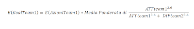
    From a formal point of view the expected number of goals is equal to the expected number of shares multiplied by the weighted average score of the probability of each action.

    We are now in the hands of these values: 2.54 goals expected for a team, 2.19 expected goals for the team 2.
    Well, but how many goals are 2:54? 3 or 2? or rather, how many times are 3 and 2? If
    are expected, are a likely outcome, I can only imagine them as means of a Gaussian distribution and group the distribution values \u200b\u200bto integers.
    A chart can better represent the concept:


    You see I made a 2:54 Gaussian with mean and standard deviation 0.60 (then the change, meanwhile, imposed this issue). Gather all probability from 1.50 to 2.50 and check the "2 goals, grouped from 2.50 to 3.50 and check out to" third goal "and so on.
    The most observant of you may have already noticed two problems: the first is not feasible five goals, one team has only four actions available, and the second is that the Gaussian has values \u200b\u200b(albeit minimal), even lower than - 0.5 and above the maximum possible value of shares + 0.5 ... then there I just have to redistribute these probabilities residual between the previous ones (simply multiply by 1 divided by the sum of the probabilities really attainable, a table will illustrate this point later).
    Do the same for the team 2. Gaussian even for him, and gather data for him. We will then
    Gaussian and we can easily see two possible outcomes.


    Now we see in the table is clear:


    first calculates the values \u200b\u200bof the goals expected from the formula above and put in the right part of the table. After which they are excluded (gray area) the probability achievable. It is therefore the sum of those achievable and we get the right values \u200b\u200bthat are 99.95% for the first team (remember the exclusion of the probability of those "five goals") and 100% for team 2.
    We then multiply the values \u200b\u200bfor the first team to 1/99.95%, and the correct values \u200b\u200bin the table on the left.

    And so a team will be able to do with his fourth goal in the shares granted
    0 0.03% of the cases indicates that P (0; team1)
    1 goal in 4.10% of the cases indicates that P (1; team1)
    2 goals in the 43.16% of the cases indicates that P (2; team1)
    3 goals in the 47.26% of the cases indicates that P (3; team1)
    4 goals in 5.45% of the cases indicates that P (4; team1 )
    the which gives the desired distribution with mean equal to 2:54 of goals and desired standard deviation 0.60

    Same thing for the team 2.

    At this point we have the chances of goals scored for each team.
    Since they are independent events we can provide considering the joint probability.
    So the probability of a tie for second at 2 is 43.13% * 57.26% = 24.69%.
    had one for 3 to 3 is 47.26% * 28.73% = 13:57%. And so on.
    So the probability of a draw P ("X") is the sum of the probability of having one of the possible draws, and then the sum of the probabilities of 0 and 0, 1 to 1 of 2 in 2, 3 to 3, 4 to 4.

    per calcolare la Probabilità di vittoria del team 1 P("1") mi basta moltiplicare le probabilità di tutti i risultati che la possano dare e quindi 1 a 0, 2 a 0, 2 a 1, 3 a 0, 3 a 1, 3 a 2, 4 a 0, 4 a 1, 4 a 2, 4 a 3. Le sommo e il gioco è fatto.
    Idem per il team 2 ed ecco i valori delle somme delle probabilità di avere "1/X/2" evidenziate in rosso nella tabella (ho tagliato la parte destra per semplicità)


    Quindi con 4 azioni al team 1 e 6 al team 2 e i valori dati di centrocampi, attacchi e difese mi aspetto il 43.80% di vittorie per il team 1, il 38.87% di pareggi e il 17.32% di vittorie per il team 2.
    In summary

    These are the values \u200b\u200bof this event. The pair of actions assigned (4, 6) occurs in 20.8% of cases, the expected goals with 2:54 and 2.19 for the first team for the second team translates into just under 44% of wins for a team, just under 39% draws and 17% of wins for team 2. Having these values \u200b\u200b
    1/X/2 .20% in 8 cases, this means that this event contributes to the total 43.80% * 8.20% = 3:59% to win by 1, to 38.87% * 8.20% = 3.18% of draws and * 8:20 to 17:32% to 2% of wins in total.
    As shown in the table:


    At this point, simply repeat the procedure per tutti gli eventi e otteniamo la tabelle:


    e


    non mi resta che sommare le celle che contengono i valori di 1/X/2 Totali per ottenere il valore finale che cercavo:


    quindi, in conclusione, prima delle modifiche con quei valori mi potevo aspettare quasi l'89% di vittorie per il team 1, il 7% di pareggi e poco meno del 4% di vittorie per il team 2.


    POST MODIFICHE

    Dopo le modifiche i casi passano da 11 a 91 e le cose si complicano un pochino.
    Niente di impossibile comunque.
    I proceeded to consider separately the data column by column, starting from the right, ie "10 actions assigned to team 2" and seeing what the results are expected for all other possible actions of the team variandi 1 (in this case 10 having the team 2, team 1 will have a variable number from 0 to 5), and then proceed to all other columns to the left.
    The analysis is broken down into 10 phases.
    For example, in the fourth column from the right we find the values \u200b\u200bseen in the example above (4 to team 1, team 6 to 2):


    grouping the 10 columns in one table we get the table of actions and goals expected:


    and the expected results, obtained as above by assessing the likelihood of 1/X/2 for each event and then multiplied by the probability of the event.


    aggregating the various phases obtained separately into the fixed number of shares for the team 2 gives the total is 90.97% of 1, 6.40% and 2.62% of X 2.
    At this point a comparison can be established before and after the change:


    with a standard deviation of the Gaussian 0.6 goals expected that the changes we see in this case, increase the% of win the strongest team, reduce ties and reduce even more the results "unexpected", that the victories of the two weakest teams: a reduction of 1.31%, -33.3% to 3.93% of the previous results "2", which were obtained previously.
    If you mean the "random" as the% of the results "unexpected" that favor the weakest team, well in that case, the numbers tell us that the "random" is (and there should be), but was reduced .

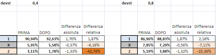
    Some may ask whether this conclusion depends on the assumed standard deviation (which is the only discretionary element in all this analysis), well then let us look at 0.4 and 0.8 instead of 0.6 and we see that


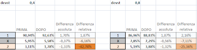
    cambiano i valori relativi, ma pochissimo quelli assoluti (i "2" si risudono del 1.33% con dev.st 0.4, del 1.31% con dev.st 0.6 e del 1.32% con dev.st 0.8).


    Naturalmente posso provare a impostare (e lo potete fare anche voi nel file allegato) dei valori di prova, per vedere come varino le probabilità di 1/X/2 tra PRIMA e DOPO le modifiche al variare delle valutazioni di campo.

    1) Pongo tutti i reparti uguali dei due team, e poi faccio crescere il centrocampo del team 1:


    nel primo caso, di completo equilibrio, vedo che si riducono le % di probabilità di vittoria per uno dei due team (da 39.56% a 38.17%) e aumentano i pareggi, del 13.40% in termini relativi (cioé sul valore precedente)
    Se aumento il CC del team 1 da 6 a 6,5 vedo che nella seconda tabellina ho ancora un aumento dei pareggi (meno rispetto al valore prededente), una sostanziale stabilità delle vittorie di 1 e una riduzione del 8.56% delle vittorie per il team più debole.
    La dinamica continua all'aumentare del valore del CC del team 1. Quindi, le MODIFICHE:
    • aumentano il numero dei pareggi in caso di partite equilibrate
    • diminuiscono il numero di vittorie "impreviste" del team più debole, e più il team è debole, più si riducono le sue chance di vittoria "imprevista"
    seem both elements on which agreement can be reached.


    *****

    Finally one may ask, "Well, we have seen what happens in terms of 1/X/2, but about the goal difference?". Yeah, one thing is a victory with three goals difference, another one with only a narrow goal.
    How to do it? Simple: the point where we took the values \u200b\u200bof the goals expected for the two teams and calculate the% chance of victory by adding the probabilities of "1 to 0" with "2 to 1", the "2 0" etc. .. . hours disaggregate wins with 1 goal difference from those with 2 goals difference, etc. ... and we get a table so as to the "primacy of Changes"


    as you see, for example, the number of wins for team 2 in the usual case (4 and 6 shares at a team shares the team 2) equal to 1.42% the total is all centered on "the victory with a goal difference", where we find a nice .27% of the occurrences. Not so, for example, for victories in a team event (7 actions to team 1 and team 3 to 2), in which case we have the fact 99.93% of wins of a team that moltipicate the probability of the event ( 24.18%) tells me that in this event are the victories of 24.16% of the total absolute event "a victory for the team", in which case the victories are made with more likely with 3 goals and 4 goal margin (9:54% and 8.14%).
    What is best seen if I apply conditional formatting to cells


    back now to the results table total


    that can also be seen in a chart with the x-axis the number of goals waste (in favor of team 1): a blue one for the team's victories, gray ties, wins in the red for the second team


    If I do the exact same procedure for the post changes (or better, 10 the same procedures, since I'll have to break up the above analysis tabellona colonna per colonna) ottengo alla fine un confronto tra PRIMA e DOPO:


    e cioé (i valori nuovi sono a destra, più scuri dei precedenti)


    • diminuiscono i rettangoli rossi dei risultati "imprevisti" di vittoria per il team 2 più debole
    • diminuiscono i pareggi
    • aumentano le vittorie del team 1 più forte attorno ai valori più probabili (2, 3, 4 gol di scarto)
    • diminuiscono le vittorie del team 1 più forte attorno ai valori meno probabili (1, 5, 6, 7 gol di scarto)
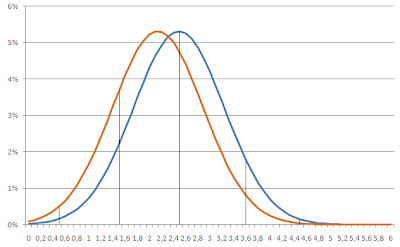
    In sostanza la curva diventa più alta e più close around the most probable values, ie reduces the variance of the curve around its average .
    If I represent the above graph as a trend I see in fact that the curve after modification, in red, compared to the curve of the PRE changes, in blue, is, as indicated by the arrows in the sides closer (decreasing the extreme results) and higher the maximum value:


    I am attaching the file.
    On the "INPUT" you can enter all the values \u200b\u200byou want and you will see:
    • in the green zone the estimate of the allocation of shares based on values \u200b\u200bentered
    • in midfield zona viola la stima dei risultati in base ai valori di attacchi e difese inseriti (e deviazione standard), con predictor base 1/X/2 e avanzato, con l'analisi dei gol di scarto. Inoltre c'è il grafico per vedere come variano le curve relative.


    QUI
    potete scaricarlo (sia per Excel nuovo che per versioni precedenti)
    http://sites.google.com/site/andreactools/home/TOOLPredictorino1.2.xlsx?attredirects=0&d=1


    Buon divertimento
    Andreac-NH

    edit: nota finale per i più pignoli -> se si pone tutto uguale tra team 1 e team 2 ci sono delle piccolissime differences between the% of goal difference to team 1 and team 2, which should be the same, I'm talking about hundredths of a percentage point. And I've split my head to find reasons, but after hours and hours of trial and I did not. These things are minor and completely irrelevant, but I wish it was all perfect. Be patient.


    PS. take a look at ' CONTENTS of the blog, there are several items that may be of interest.


    Andreace (team in Hattrick ID 1730726)

    Creative Commons License
    by
    This work is licensed under Andreace a Creative Commons Attribution-Noncommercial 3.0 Unported License . Ie, this work may be freely copied, distributed or modified without the express permission of the author, provided that the author is clearly stated and the publication is not for commercial purposes.

    Friday, September 24, 2010

    Can You Return Xbox Live Cards To Cvs

    Hattrick - Money


    I wanted to go on a talk started a couple of months ago in this article
    http://acandio.blogspot.com/ 2010/07/hattrick-equilibri-finanziari-il.html
    to make a few reflections on the economic management team. Not These "certain laws", only that I want to share personal ideas.

    As seen in that the only sources of revenue for your company are
    • Collections viewers
    • SPONSOR
    • Proceeds of sale of players
    seen as the first two grow quite content, and then to grow faster than you just have to rely on the sale of players.
    If, like me, you are not traders and manage your team with a limited number of market transactions, then you just need to maximize your pink. How to do it?
    Let's see if I can explain my point of view.


    IL SINGOLO GIOCATORE

    Innanzitutto devo considerare quali fattori incidono sul prezzo del giocatore (indico in grigio le caratteristiche del giocatore su cui non abbiamo alcun potere di modifica, in azzurro gli elementi su cui abbiamo un potere di intervento limitato, in verde quelli che possiamo direttamente modificare):
    • Età
    • Livello di Forma
    • Livello di Resistenza
    • Livello di Esperienza
    • in misura minore il carattere ( Simpatia, Aggressività, Condotta morale) e in certi casi also the charisma
    • Nationality
    • Specialty Level (and decimal) of the skill level of the primary
    • secondary skills relating to the role
    • Seasonal variations Market
    • external shocks (the HT editorial)
    The Age (and you must keep in mind not only years but also the day) is partially outside of our control, inexorably aging player, but we can decide when to put it on sale.
    Form is marked in blue as it can affect the general training, but this workout, as mentioned by HT, it will be removed in the future and then will be placed outside the control of managers.
    On Resistance can dip into, but it is a key element in the transaction. Sull'Esperienza have power to amend in the sense that we do play more and gain more experience, but practically only in the case of the "future coach" is a crucial phase in the market.
    on character, charisma, national and, especially, we can not do anything, as is born, it dies and the player is not in our control. On
    level of primary and secondary hand engrave with the training.
    The cyclical variations of the market enable us, if we can take advantage of it, to obtain rates. On external shocks, such as the HT editorial that touch on elements such as the contributions of certain roles or the speed of training we can do nothing, alas, only to suffer.

    In essence, what is there to act upon? four parameters, number 1) to 4)
    1. Age (not only years, even days)
    2. level (and decimal) of the main skill
    3. level of skill on the secondary role
    4. Seasonal variations Market
    's simple, studying the "compare transfers" (" CT) of the players on sale of building tabelle con cui studiare come varino i prezzi al variare di questi elementi.
    Naturalmente occorre ricordare che il CT mette assieme giocatori che hanno 17 anni e 1 giorno con quelli che ne hanno 17 e 111 giorni, giocatori con specialità e giocatori senza, giocatori più o meno in forma, giocatori con molti decimali e giocatori appena scattati. Un calderone in cui vanno a finire giocatori diversissimi e quindi la media è solo un valore di riferimento approssimato. Tuttavia, per quanto impreciso, tale valore fa da riferimento per gli scambi successivi e quindi è un parametro da considerare con la massima attenzione.

    Prendiamo un Difensore Centrale e vediamo come varino i prezzi in funzione dei parametri 1) e 2), cioé di età and skill level of the primary, taking the fixed 3) (4 in the secondary direction and the other skills <= a 4, e naturalmente) e il 4), l'analisi è cioé fatta ora e i prezzi saranno diversi da quelli di due settimane fa o di quelli che ci saranno tra due settimane. Si tratta solo di un abbozzo, ma utile per rendere l'idea.


    Table 1: Prices vary on the player's age and skill level of the primary defense, secondary constants (directed = 4, other <= a 4)

    Thus we see as acceptable in a 17-year-old defense, with four in the control room is traded on the 20k. A good 17-year-old still on 90k, an excellent 360k and so on.

    Let 2 forces in action:
    • The primary change in SKILL , denoted by dS (difference of skill), it shows me what is re-evaluating the player for taking a picture skill. So for the 17 year old: 90-20 = 70K for a good shot, 360-90 = 270k per click to excellent ... etc. Here is a zoom of the previous table that shows me that I see these changes in the lines:


    I can make a table that shows me these values:

    Table 2: gains due to dS ' increase in primary skill of the player

    The change in price variation of skill is, in this table is always positive: the increase in these levels of skill always generates an increase in price (not always the case, for high values \u200b\u200bof skill, such as over 16 the rise of the stipendi tende a provocare riduzioni di prezzo all'aumentare del livello di skill).
    Per inciso potremmo dividere tali valori per il numero di settimane che occorrono allo scatto di skill per vedere la resa settimanale, cioè considerare il rapporto dS/settimane necessarie per lo scatto (dato che ad esempio guadagnare 400k con uno scatto che necessita di 4 settimane di allenamento rende 100k a settimana, meglio di guadagnare 600k con uno scatto che ne necessita 8 e rende quindi 600/8=75k a settimana)

    Tabella 3: resa settimanale dell'allenamento (dS/settimane necessarie)

    Vedete ad esempio come per un 21 enne lo scatto 8 to 9 in defense takes the player from 190k to 555k of value (see Table 1) making a profit of 555-190 = 365k (see Table 2), requiring weeks of training allows a 5:36 guagagno weekly 365k/5.36 = 68.1k weekly. Train a 21-year-old from 12 to 13 ports in defending the player from 1900k to 2430k in value (see Table 1) making a profit of 530k = 2430-1900 (see Table 2), requiring 30.8 weeks of training allows a weekly guagagno 530k / = 63.8k 8.30 per week, less than the previous year. Of course, in these weeks we will have players level much higher than before.


    All this is of course if the player in the meantime, a birthday, otherwise we consider the second force in action:
    • The Age variation, denoted by dE (age difference), it shows me what is re-evaluating or devalues \u200b\u200bthe player for taking skill. If we look in Table 1 above we see how good that makes 18y.o. changed from a CT value of 90k to 45k, halving its value. If it were excellent would increase from 360k to 255k, 105k losing. Here is a zoom of Table 1 shows these changes that I see in the columns

    This table

    Table 4: Changes in the value of the player after dE aging

    see the devaluations and revaluations in the red to blue. It may seem strange, but it happens that a player who is older rivals. Sometimes even consistently: an extraordinary 21 years and 111 days worth 860k in CT, the day after that is 1000k ... 140k a day doing nothing, not bad.
    are elements to keep in account: if you take a beautiful 18 year old with many days at 2200K and trained hard, I found a wonderful 19 years with a value of 2035k. Not a good deal.


    So it should be noted if the current price of the player, which indicates how PATT , equal to the purchase price pACQ with changes of skill and age dS dE is or is not greater than the purchase price. So if

    PATT = pACQ + + dS dE> pACQ

    In view of the magnificent 19 year old is 2035 +635 = 2200 - 800> 2200 that is false, because dE = 800 is greater of dS = 635. Indeed

    pACQ + + dS dE> pACQ can be reduced to dS + dE> 0

    the sum of the changes affected the price of the player must be a positive example not seen it is because the depreciation dE is higher than the gain from skill-up dS.


    Now the speech should extend also to the secondary, we could build the same tables and study the variations in prices of primary defense lawyers with skills from 6 to 16 and ages 17 to 23 from a level 4 of a director a level 5 and above. I point this difference ds (difference of secondary, "S" capitalized). Without post tables on tables at the end conclude that the sum total of variations must be positive for a gain.

    Ditto if we extend the analysis to collect prices week after week. The change in the market must be dM inserita nell'analisi.

    Alla fine otterremo che per avere un guadagno deve essere

    dE + dS + ds + dM > 0


    Ci sono quindi 4 modi per avere un guadagno (conservo l'ordine dei numeri messi sopra degli elementi su cui possiamo agire):
    1. dE rivalutazioni del giocatore in seguito all'invecchiamento, " Age Trading "
    2. dS rivalutazioni del giocatore in seguito allo scatto di skill primaria, " Skill Trading "
    3. ds revaluation of the player following the release of secondary skills, "Trading Secondary Skill", if combined with the previous one speaks of "Bi-skillaggio" or "Tri-skillaggio"
    4. dM revaluations player after market performance, " Season Trading "
    course the effect will be the sum of all these elements, which usually positive value for changes in skills, tends to negative changes in age and cyclical than the seasonal market.
    There is of course a fifth way to make a profit when you can sell at a higher price to what you bought despite not having changed none of the four elements above. This mode is typical of pure trader is established (although now improperly) "Trading Day . Not deal here with pure trading, as mentioned above, I mention only for the sake of completeness.


    TEAM

    But now we move from the standpoint of the individual player to the team as a whole. Let's take a look at the balance sheet of the team: your ACTIVE consists of only two items: the money you have in Fund and the total value of your short list of players (the "total price" of the TEAM, pTEAM ).


    The value of the rose pTEAM is the sum of current prices PATT of all components of the rose. If the components are n, then

    which means that the value of your team is nothing more than the sum of the prices at which you bought all your players, the more the individual changes occurring as a result of advancing age, changes skills of primary and secondary market trends.

    This is a point to make: what matters is not how much you earn with the skill of your trading allenandi, what counts is the total Asset . You can also gain from the sale of 1000k a great coach fired, but in the meantime if your players are depreciated 4 of the 250k a total value of your assets does not change one iota.
    and the assets and the key to the growth of your team.

    If the business grows a little, then tomorrow we will have very little money available to strengthen our team, if it grows back much as we need to grow fast and we aim first to ambitious targets. How

    varies the activity? Simple. Just look at the formula and see item by item: The Case
    • not affected (affected with a very limited accountants who have been recently deleted) money held in cash are unproductive, do not help the growth
    • Asset Purchase prices pACQ are historical and therefore fixed.
    • the price changes of each player as a result of aging dE (usually a depreciation, negative)
    • the price changes of each player's skill as a result of growth of primary dS (usually an appreciation, positive )
    • the price changes of each player's skill as a result of growth of secondary ds (usually an appreciation, positive)
    • the price changes of each player as a result of market trends dM (cyclic)

    To analyze the set of players distinguish two groups of players:
    1. k players who receive some kind of skill training in primary or secondary ( that indicates " GALL "trained players)
    2. nk players who do not receive training in primary or secondary skill ( that indicates" gnon-ALL "untrained players)
    For example, if I give defense training to 10 players (k = 10) and I have a shortlist of 25 players (N = 25) k = 10 players I have coached (Gallo) and nk = 25-10 = 15 players untrained (gnon-ALL)

    So the change in the asset is given by two elements:

    1. the first is the sum of changes in value of trained (due to depreciation for age, skill growth and variations of primary and secondary market)
    2. the second is the sum of the changes in the value of the untrained (and their depreciation with age changes in the market).

    E 'is evident as the first element to drive the growth of the team, as the latter tends to be negative and therefore a burden that slows down the process growth. The only thing we can do to make the second element is positive (or less negative as possible) is to try to choose non-coached players who have little depreciation (low dE ) and buy them in times of low market (for a dM favorable ).
    These considerations apply of course also for allenandi, for which the depreciation will be an eye dE and market phase dM earnings and the other directed by Allen and dS ds .

    For the most growth possible I will have to allocate the resources of the team in the most profitable as possible. Given that the untrained do not guarantee growth, indeed, the brake, the ideal would be possible to target the greater% of the budget in the trained (by the way someone might argue that even the untrained indirectly contribute to the growth of the team, as good performance Team sports may contribute to good results, many fans, promotions, etc., true, but remember that the increase in the budget items to collect tickets and sponsor of the stadium is very slow).

    Of course the point is not that "most are trained, the greater the team," because as we saw in the article, the market recognizes a sorta di "resa implicita dell'allenamento" che tendenzialmente pareggia gli introiti dei diversi tipi di allenamento. Ad esempio se alleno 10 difensori (k=10) il mercato valuta per ognuno un aumento virtuale di circa 40k di valore ad allenamento (dS=40k), con un amumento totale di k*dS = 10*40k = 400k. Se alleno parate, alleno 2 giocatori (k=2) e il mercato valuta per ognuno un aumento di circa 200k di valore ad allenamento (dS=200k), per cui k*dS = 2*200k = 400k. Questo è vero tendenzialmente, in realtà i k*dS sono un po' diversi e quindi ci sono allenamenti un po' più convenienti e altri meno.


    Quindi, riassumendo, a cosa be careful to ensure greater asset growth of the team?
    • allocate the smallest possible part of the budget unproductive uses such as cash (the money we make the mold, unless you wait for more favorable market conditions) or the untrained (which often have negative balance, subtracting the total value of Assets as a result of aging). The higher the ratio Gallen / gnon-ALL greater the value growth of our team (please note that if instead of training only in primary skill train in secondary skills, then increase the value of this ratio: for example, if train parades and also give some training ride defense to my goalkeepers then this training will also benefit from the outfield players will go to defense position in the slot and will increase the range of even partially trained. Clearly this will make sense if the benefits in these weeks of training in secondary and primary gatekeepers to the defenders normal outweigh the disadvantages of not coaching the goalkeepers still in primary).
    • choose allenandi and untrained children who have impairments due to aging (minimizes dE), even better if I can find players who enjoy getting older (not done at random, must be studied well natural market to produce tables such as Table 4 above)
    • allenandi buy and no training during favorable market to minimize dM (and here it is necessary to study the market well)
    • study to pp rofonditamente the market with cross-tables "Age / level of skill primary" as seen in Table 1 above to find the dS more favorable (Table 2) in order to train the players primary skill in the shots of the most profitable (of course will not be considered dS absolutes, but the ratio dS / week necessary for the shot seen in Table 3)
    • study to pp rofonditamente the market with cross-tables "Age / secondary level of skill" to see whether or not to give the player the convenience of increases in secondary ds , of \u200b\u200bcourse, here must be regarded as the ratio ds / week needed for the shot and evaluate the potential profitability of a bi-or tri skillaggio player.


    PS. take a look at ' CONTENTS blog, there are several items that may be of interest.


    Andreace (team in Hattrick ID 1730726)

    Creative Commons License
    This work is licensed by Andreace under a Creative Commons Attribution-Noncommercial 3.0 Unported License . Ie, this work may be freely copied, distributed or modified without the express permission of the author, provided that the author is clearly stated and the publication is not for commercial purposes.