second draft
-Aug-asked me in Italy Forum
"because instead of using simulations to calculate the probability value? Remove all doubt on the sample used, no?"
Right.
Then proceed.
Meanwhile, an introduction, by http://www.liceofoscarini.it/studenti/probabilita/binomiale.html .
is an exhortation: If there are no formulas to understand, do not worry, go beyond just understanding the meaning of the speech.
The BINOMIAL
How many times have you ever play heads or tails? Surely many
. What they may not have ever thought is to find a method to determine the exact probability that a given number of shots, there is a certain amount of success (ie, heads or crosses, depending on your point of view). If we assume that the event head (0 ) is equally likely cross the event ( 1), that their chances are worth both 12:50 (50%), two launches, the probability of two crosses, eg., will be:
00:50 12:50 = 0.25 ×
Suppose now that the two events are equally likely not and that the launches are any number N . Let's also say that the successes are any number k .
The problem becomes more complicated.This is a Bernoulli scheme that has, in essence, the following features:
- each test is a random experiment that may have only two possible outcomes, with probabilities p and q = 1-p ;
- each test is performed independent of any other evidence and, therefore, in each trial the probability of success is p constant.
The probability that n on all independent tests conducted under the same conditions, we have k successes with <=n k is:
 where X indicates the random variable that counts the number of successes, p the probability of each event E , constant in all tests, and q the probability of not (E) , then q = 1-p
 I the symbol "!" is the factorial, is simple, it is the product of a number with him less than whole numbers, so if n is 4, then n! is 4 * 3 * 2 * 1 = 24. That's it.
in Hattrick, before Editing
This distribution, known as the binomial, is perfect to describe the probability distribution of the shares granted in the first hattrick of the changes, since each assignment is independent of the action below and the probability is constant, the ratio between the cube of a midfield and the sum of two cubes of the midfield.
Then the probability distribution in Hattrick was
 since n = 10 the number of shares granted and the rest comes by itself.
 In Excel the formula becomes, if you want to try,
= (FACT (10) / (FACT (k) * FACT (10-k )))*(( CC1 ^ 3 / (3 + CC2 CC1 ^ ^ 3)) ^ k) * ((CC2 ^ 3 / (CC1 CC2 ^ 3 + ^ 3)) ^ (10-k))
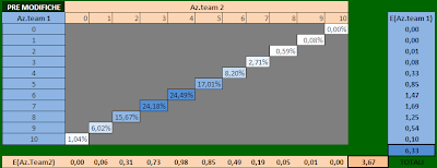
Così, se, ad esempio, il team 1 ha un centrocampo che vale 6 e il team 2 un centrocampo che vale 5, allora si fa presto a calcolare le probabilità di avere un certo numero di azioni per ogni team:
 Quindi se i centrocampi hanno quei valori il team 1 avrà il 17.01% di probabilità di avere 5 azioni, il 24.49% di averne 6, il 24.18% di averne 7 eccetera...
 Mi direte, ok, ma quante azioni si aspetta di avere il team 1 in totale?
Per sapere tale valore devo introdurre il concetto di speranza matematica (o " valore atteso "): niente di difficile anche qui, mettiamo che in un gioco abbiate 25% chance of winning € 100 and 75% chance of winning € 200, then your expected payout is 0.25 * 100 +0.75 * 200 = 175 €. There is a case in which they win € 175, but if you play 10 times you will tend to win € 1750 with a win "average" of 175 € to play.
Returning to our actions then just multiply the% of action to have the number of shares granted, which measures expectations for the team 1 (indicated by "E (Az.Team1), where E stands for Expected, "expected" if I remember correctly) and the second team are:
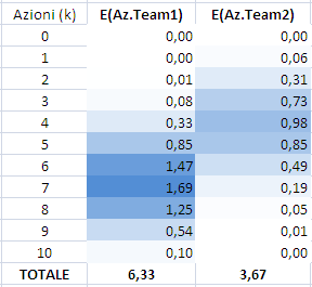
then just do the sum to see if my midfield is 6 and the opponent's 5, then I will have an expected number of shares equal to 6.33 and 3.67 of my opponent.
This is not a sample, but by the law of binomial probability.
As you can see the relationship between my actions and those of the opponent is expected
then in that case is expected that the My actions are the 172.8% of the opponent.
This value coincides with that found in the first part of this, the value of "fair" allocation of shares (the ratio of the cubes of midfield), in fact
Now, we can think of to fix the value of the midfield in the second team (my opponent) to "5" and then change the value of my team's midfield " CC1 " from "1" to "9" to see how to vary the odds of having a certain number of shares
This is not a sample, but by the law of binomial probability.
As you can see the relationship between my actions and those of the opponent is expected
E (Az.Team1) / E (Az.Team2) = 6:33 / 3.67 = 1728
then in that case is expected that the My actions are the 172.8% of the opponent.
This value coincides with that found in the first part of this, the value of "fair" allocation of shares (the ratio of the cubes of midfield), in fact
^ 3 CC1 / CC2 ^ 3 = 6 ^ 3 / 5 ^ 3 = (6 * 6 * 6) / (5 * 5 * 5) = 216/125 = 1728
Now, we can think of to fix the value of the midfield in the second team (my opponent) to "5" and then change the value of my team's midfield " CC1 " from "1" to "9" to see how to vary the odds of having a certain number of shares

and actions expected total:

I can represent a graph
 take the expected actions shaped, slightly "S" shaped, with inflection point at the point where the same values \u200b\u200bof the two midfield, CC1 = CC2 = 5.
 Now we know how to vary the actions expected of a team to change his midfield, but since we know that the total amount have to be 10, you also know the expectations of those two teams. In
formula E (Az.Team2) = 10 - E (Az.Team1), and then we can calculate what interests us, namely, the relationship between the actions assigned to the team and assigned to a team of 2 to change the team's midfield 1:

Just for reference as you see in the "6" to find the values \u200b\u200b6.33 and 3.67 seen before 1728 and their relationship, that is 172.8%.
in Hattrick, AFTER the Changes
not more than 10 shares "common" in which whoever wins if he takes her home, but my 5 exclusive five municipalities in which the action is or is lost or my and my opponent's 5 exclusive or where are his or lost.
How does the law of probability? The laws vary
, step by step procedure to analyze: we focus our attention not so much on the actions of a team and those of two separate teams, but consider them together, seeing which pairs (Actions for Team 1, Actions for Team 2) can be obtained.
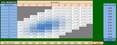
Before these changes could be pairs of actions
(0, 10) or (1, 9), (2, 8), (3, 7), (4, 6), (5, 5), (6, 4), (7, 3), (8, 2), (9, 1), (10, 0)
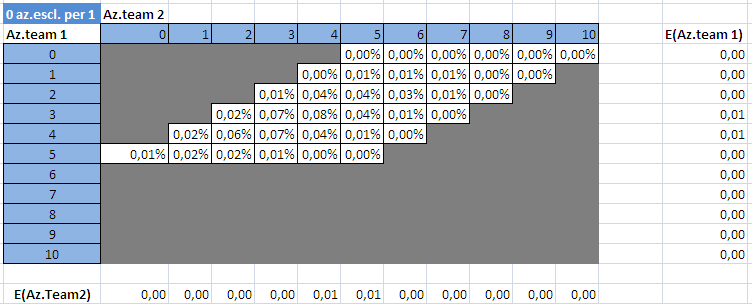
and is easy to calculate a table that reflects these possibilities and their% probability according to the binomial :
course of action possible pairs are arranged in diagonal, because the more shares the other has a less and vice versa. You see that line by line you can see the expectations for the team shares a column by column and those expected for the second team.
And after the changes?
Well I confess that I had to think we all yesterday, but eventually I did. Here's the solution.
First, consider the actions.
For them is the classic view of the binomial above, except that the shares to be allotted are 5 and 10

so everything is easy: a total of 3.17 shares expectations for the team 1 (sum of column E (Az.Team 1) 1.83 and waited for the team 2 (sum of row E (Az.Team 2))
I continue with the exclusive actions.
same law of probability, except that the shares would not be assigned missing. So for a team that is This table (which can be summed up in one column)

while the second is this team (which can be summarized in the line)

now see that the total number of shares expected to Team 1 and Team 2 is the same in both common in the exclusive, but change the "couples". Now it is possible that the first couple were not. The difficult point was how to integrate the table of probabilities of joint actions with the column of probabililtà exclusives for the team and the first row of the probability of exclusive 2 for the team.
These events are independent then the joint probability is given by the multiplication of the probabilities of single events. I proceeded to the sum of conditional probabilities, but I think it's clearer if I explain step by step.
I started considering the event (0, 5) in the table of actions.
This event occurs in 0.66% dei casi.
Ora ipotizzo che nelle sue azioni esclusive il team 1 non vinca neanche un'azione (sia Az.team 1 = 0), evento che si realizza anche esso nel 0.66% dei casi.
Passo infine alle azioni del team 2, il quale può ottenere da 0 a 5 delle sue azioni esclusive, con le probabilità viste nella riga sopra. Ne ottiene 0 col 10.20% di possibilità.
In tal caso vale (0;5) + 0 azioni per il team 1 + 0 azioni per il team 2, resta (0;5) con una probabilità di 0.66% (dalla tabella delle azioni COMUNI) moltiplicata per il 0,66% (probabilità di nessuna azioni esclusive per il team 1) e per il 10.20% (porbabilità di 0 azioni esclusive per il team 2) che fa il 0.000447% totale.
So I can calculate the probabilities of events (0, 5) to (0, 10), varying the% of the shares exclusive 2 for the team, if a team does not get any of his actions exclusive
P ( 0, 5) = 0.66% * 0.66% * 10.20% = 0.000447%
P (0, 6) = 0.66% * 0.66% * 29.51% = 0.001293%
P (0, 7) = 0.66% * 0.66% * 34.15 % = 0.001496%
P (0, 8) = 0.66% * 0.66% * 19.76% = 0.000866%
P (0, 9) = 0.66% * 0.66% * 5.72% = 0.000251%
P (0, 10) = 0.66% * 0.66% * 0.66% = 0.000029%
in table

proceed similarly for the successive values \u200b\u200bof the diagonal of common shares multiplied by the 0% chance of actions unique to the team and for 1% probability of action 2 exclusive for the team, identified the% probability of pairs of values \u200b\u200b(Az 1 team, az. team 2) while holding that a team does not get any action exclusively.
I get the following table:

A similar assumption is that the team gets a first action of its exclusive. Keeping everything else unchanged (do not change the probability of joint actions, nor those who are excluded for the team 2) I get the following table:
 see that:
 se sono 3

se sono 4

o se sono 5

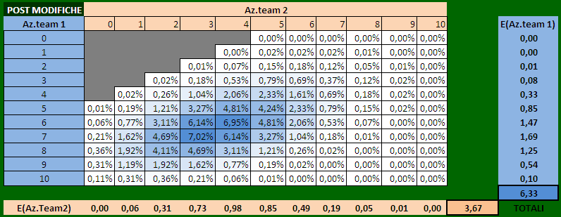
Non resta che fare la somma, casella per casella delle precedenti 6 tabelle e otteniamo la probabilità totale delle coppie di azioni
then here is the coveted table of possible pairs of% of shares allocated to the two teams. With a hint of
jo76_it tool can be seen in how the distribution of the total shares allocated in total: just make the sum of the diagonals and you see what is to have 5% shares, have 6, etc. ... (See the image diagonal of 15 shares)
The distribution is (and not surprising) in the form of a Gaussian.

You want excel to do some 'testing the variation of the midfield? I thought so.
Here it is.
To my knowledge this is the 'only tool that is able to estimate the% of pairs of possible actions. after the changes. An essential element if you want to build a tool to make some estimates of the lot. I left it open so that we can play around as best you are comfortable because of that.
I close the parenthesis: if you look at the line of the Shares waited for Team 2 and the column of those expected for a team that you see are the same, identical to the first of the changes. Ditto for the totals.
Ma allora non cambia nulla?
Non cambierebbe nulla se fosse possibile assegnare un numero "continuo" di azioni, cioè se fosse possibile assegnarne 6.33 al team 1 e 3.67 al team 2. Così non è e ai due team vengono assegnate un numero discreto di azioni (1, 2, 3, ecc)
La differenza sta appunto nella CONVERSIONE di quei valori attesi in azioni concrete ai due team.
Come visto, da un punto di vista numerico:
in Hattrick, AFTER the Changes
not more than 10 shares "common" in which whoever wins if he takes her home, but my 5 exclusive five municipalities in which the action is or is lost or my and my opponent's 5 exclusive or where are his or lost.
How does the law of probability? The laws vary
, step by step procedure to analyze: we focus our attention not so much on the actions of a team and those of two separate teams, but consider them together, seeing which pairs (Actions for Team 1, Actions for Team 2) can be obtained.
Before these changes could be pairs of actions
(0, 10) or (1, 9), (2, 8), (3, 7), (4, 6), (5, 5), (6, 4), (7, 3), (8, 2), (9, 1), (10, 0)
and is easy to calculate a table that reflects these possibilities and their% probability according to the binomial :

course of action possible pairs are arranged in diagonal, because the more shares the other has a less and vice versa. You see that line by line you can see the expectations for the team shares a column by column and those expected for the second team.
And after the changes?
Well I confess that I had to think we all yesterday, but eventually I did. Here's the solution.
First, consider the actions.
For them is the classic view of the binomial above, except that the shares to be allotted are 5 and 10

so everything is easy: a total of 3.17 shares expectations for the team 1 (sum of column E (Az.Team 1) 1.83 and waited for the team 2 (sum of row E (Az.Team 2))
I continue with the exclusive actions.
same law of probability, except that the shares would not be assigned missing. So for a team that is This table (which can be summed up in one column)

while the second is this team (which can be summarized in the line)

now see that the total number of shares expected to Team 1 and Team 2 is the same in both common in the exclusive, but change the "couples". Now it is possible that the first couple were not. The difficult point was how to integrate the table of probabilities of joint actions with the column of probabililtà exclusives for the team and the first row of the probability of exclusive 2 for the team.
These events are independent then the joint probability is given by the multiplication of the probabilities of single events. I proceeded to the sum of conditional probabilities, but I think it's clearer if I explain step by step.
I started considering the event (0, 5) in the table of actions.
This event occurs in 0.66% dei casi.
Ora ipotizzo che nelle sue azioni esclusive il team 1 non vinca neanche un'azione (sia Az.team 1 = 0), evento che si realizza anche esso nel 0.66% dei casi.
Passo infine alle azioni del team 2, il quale può ottenere da 0 a 5 delle sue azioni esclusive, con le probabilità viste nella riga sopra. Ne ottiene 0 col 10.20% di possibilità.
In tal caso vale (0;5) + 0 azioni per il team 1 + 0 azioni per il team 2, resta (0;5) con una probabilità di 0.66% (dalla tabella delle azioni COMUNI) moltiplicata per il 0,66% (probabilità di nessuna azioni esclusive per il team 1) e per il 10.20% (porbabilità di 0 azioni esclusive per il team 2) che fa il 0.000447% totale.
So I can calculate the probabilities of events (0, 5) to (0, 10), varying the% of the shares exclusive 2 for the team, if a team does not get any of his actions exclusive
P ( 0, 5) = 0.66% * 0.66% * 10.20% = 0.000447%
P (0, 6) = 0.66% * 0.66% * 29.51% = 0.001293%
P (0, 7) = 0.66% * 0.66% * 34.15 % = 0.001496%
P (0, 8) = 0.66% * 0.66% * 19.76% = 0.000866%
P (0, 9) = 0.66% * 0.66% * 5.72% = 0.000251%
P (0, 10) = 0.66% * 0.66% * 0.66% = 0.000029%
in table

proceed similarly for the successive values \u200b\u200bof the diagonal of common shares multiplied by the 0% chance of actions unique to the team and for 1% probability of action 2 exclusive for the team, identified the% probability of pairs of values \u200b\u200b(Az 1 team, az. team 2) while holding that a team does not get any action exclusively.
I get the following table:
A similar assumption is that the team gets a first action of its exclusive. Keeping everything else unchanged (do not change the probability of joint actions, nor those who are excluded for the team 2) I get the following table:
 see that:
 - values \u200b\u200bare higher, infatti la probabilità che il team 1 ottenga 1 azione esclusiva è 5.72%, e non più lo 0,66% di averne 0
- le coppie risultano spostate in basso di una riga, infatti se il team1 ottiene 1 azione esclusiva, l'evento (0;5) diventa (1;5) e quindi tutto si sposta in basso di 1 riga.
 se sono 3
se sono 4

o se sono 5

Non resta che fare la somma, casella per casella delle precedenti 6 tabelle e otteniamo la probabilità totale delle coppie di azioni

then here is the coveted table of possible pairs of% of shares allocated to the two teams. With a hint of
jo76_it tool can be seen in how the distribution of the total shares allocated in total: just make the sum of the diagonals and you see what is to have 5% shares, have 6, etc. ... (See the image diagonal of 15 shares)
The distribution is (and not surprising) in the form of a Gaussian.

You want excel to do some 'testing the variation of the midfield? I thought so.
Here it is.
For Excel 2007: https: / / sites.google.com/site/andreactools/home/TOOLAssegnazioneAzioni1.1.xlsx? Attredirects = 0 & d = 1
for Excel 1997-2003: https: / / sites.google.com/site/andreactools/home/TOOLAssegnazioneAzioni1.1.xls? Attredirects = 0 & d = 1
To my knowledge this is the 'only tool that is able to estimate the% of pairs of possible actions. after the changes. An essential element if you want to build a tool to make some estimates of the lot. I left it open so that we can play around as best you are comfortable because of that.
I close the parenthesis: if you look at the line of the Shares waited for Team 2 and the column of those expected for a team that you see are the same, identical to the first of the changes. Ditto for the totals.
Ma allora non cambia nulla?
Non cambierebbe nulla se fosse possibile assegnare un numero "continuo" di azioni, cioè se fosse possibile assegnarne 6.33 al team 1 e 3.67 al team 2. Così non è e ai due team vengono assegnate un numero discreto di azioni (1, 2, 3, ecc)
La differenza sta appunto nella CONVERSIONE di quei valori attesi in azioni concrete ai due team.
Come visto, da un punto di vista numerico:
- PRE modifiche: se le azioni del team 1 sono X allora quelle del team 2 sono (10-X)
- POST modifiche: se le azioni del team 1 sono X allora quelle del team 2 sono un numero variabile tra 0 e Min(10;15-X ) , col vincolo che la somma sia almeno pari a 5 (le azioni comuni che devono comunque essere assegnate)
E questo come incide?
Incide nel seguente modo.
Consideriamo il primo esempio visto in alto, CC1=6 e CC2=5, allora in tal caso l'assegnazione equa vorrebbe che il team 1 avesse il 172.8% di azioni del team 2.
Prima delle modifiche era possibile solo la combinazione "6 al team 1 e 4 al team 2" che dava al team 1 il 150% di azioni rispetto al team 2. Oppure "7 al team 1 e 3 al team 2" che dava al team 1 il 233% di azioni rispetto al team 2. Non si riusciva ad avvicinarsi al valore equo di 172.8%.
Dopo changes however you can, for example, the combination "7 to 1 and 4 team to team 2", which gave the team a 175% share compared to team 2. A value very close to 172.8% of the fair!
This illustrative table:

We have the values \u200b\u200bof fair allocations of shares between team 1 and team 2 with the variation of a midfield team. So let's see what were the combinations of actions to the two teams that are closest to fair value.

I marked in red when the number of shares varies (after editing), allowing a relationship of allocation of shares between the two teams closest to the fair.
fact the values \u200b\u200bof (Az.Team1) / (Az.Team2) after the changes are almost always closer to the value E (Az.Team1) / E (Az.Team2). The testimony comes from the numerical value of standard deviation than the fair value of the distortions that almost halved: from 00:27 to 12:15.
I hope with this to have made a contribution with respect to the statistically based random allocation of shares before and after the change.
PS. take a look at ' CONTENTS of the blog, there are several items that may be of interest.
Andreace (team in Hattrick ID 1730726)
Andreace (team in Hattrick ID 1730726)

This work is licensed by Andreace under a Creative Commons Attribution-Noncommercial 3.0 Unported License . Ie, this work may be freely copied, distributed or modified without the express permission of the author, provided that the author is clearly stated and the publication is not for commercial purposes.
0 comments:
Post a Comment